Q learning Notes
What is Q?
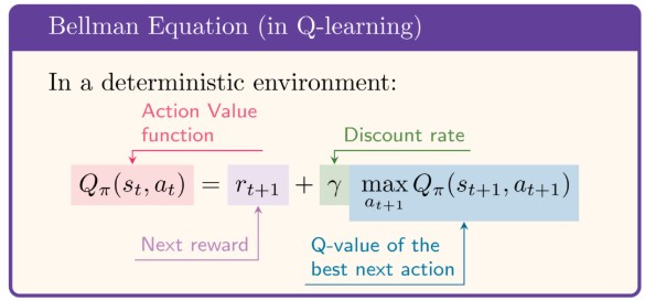
Action value function $Q(s,a)$ associating a value (reward) to any combination of state $s_t$ and action $a_t$.

Recursive definition of Q
$Q(s_t,a_t)$ can be written as a recursive formula called the Bellman equation, expressing the Q value in the current state in terms of the Q values of the next states:
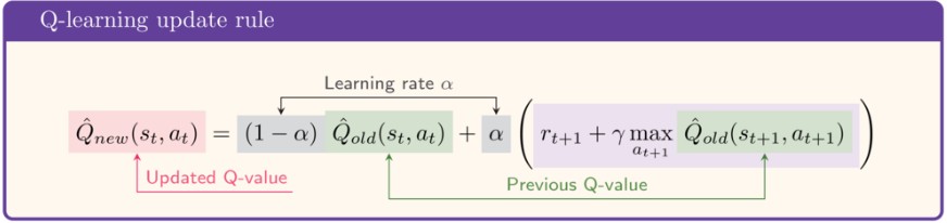
The update rule for Q learning -
Q Network - QN
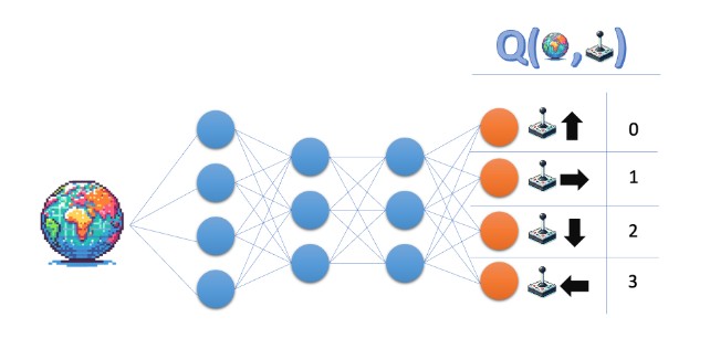
Mapping states to action values
Q-network maps state -> Q-values for all actions, that are possible from that state.
The output depends on the number of actions and number of states.
So for 5 input states, we get 5 rows, each row has 4 actions values (one per action).
- If action space has 4 actions:
- input one state tensor (state_dim,) -> output (4,) : 1 dimension vector
- input batch of 5 states (5, state_dim) -> output(5,4) : 2 dimension matrix
- NN’s Output index corresponds to the action ID.
if the output of the network is [q0,q1,q2,q3]. That means :- q0 = Q(s, action 0)
- q1 = Q(s, action 1)
- etc.
argmaxpicks the idex of highest Q-value, and that index is the action we send to env.step(action).
Bellman optimality equation (for $Q^{*}$):
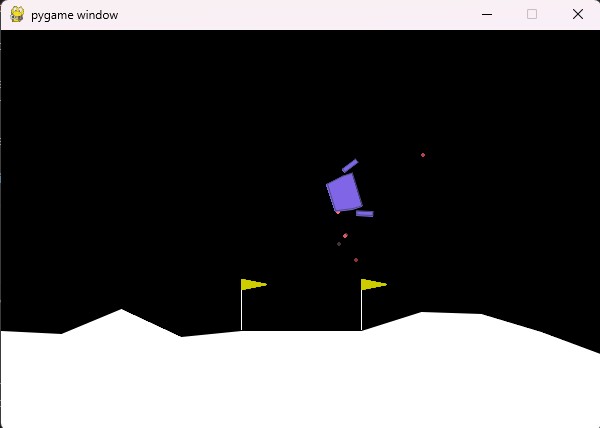
A neural network to implement the Q function for Lunar Lander environment
# QNetwork(state_size, action_size). for Lunar Lander action_size = 4
# Action space - [0, 1, 2, 3] - [do nothing, fire left engine, fire main engine, fire right engine]
# State space - 8 dimensions - [x, y, x_dot, y_dot, angle, angular_velocity, left_leg_contact, right_leg_contact]
import torch
import torch.nn as nn


class QNetwork(nn.Module):
    def __init__(self, state_dim, action_dim):
        super(QNetwork, self).__init__()
        self.fc1 = nn.Linear(state_dim, 64)
        # two fully connected hidden layers with 64 nodes each
        self.fc2 = nn.Linear(64, 64)
        self.fc3 = nn.Linear(64, action_dim)

    def forward(self, x):
        if not isinstance(x, torch.Tensor):
            x = torch.tensor(x, dtype=torch.float32)
        x = x.float()
        x = torch.relu(self.fc1(x))
        x = torch.relu(self.fc2(x))
        return self.fc3(x)
Training the neural network with lunar lander environment - Part 1
"""
Simple LunarLander DQN-style training loop.
"""

import gymnasium as gym
import torch
import torch.nn as nn

from q_network import QNetwork

GAMMA = 0.99
LR = 1e-4
NUM_EPISODES = 10


model = QNetwork(8, 4)
optimizer = torch.optim.Adam(model.parameters(), lr=LR)
criterion = nn.MSELoss()


def to_tensor(state):
    return torch.tensor(state, dtype=torch.float32)


def select_action(net, state_tensor):
    q_values = net(state_tensor)
    return torch.argmax(q_values).item()


def calculate_loss(net, state, action, next_state, reward, done):
    state_t = to_tensor(state)
    next_state_t = to_tensor(next_state)

    q_values = net(state_t)
    current_q = q_values[action]

    with torch.no_grad():
        next_q = net(next_state_t).max()
        target_q = reward + GAMMA * next_q * (1 - int(done))

    return criterion(current_q, target_q)


env = gym.make("LunarLander-v3", render_mode="human")

for episode in range(NUM_EPISODES):
    state, _ = env.reset()
    done = False
    episode_reward = 0.0

    while not done:
        action = select_action(model, to_tensor(state))
        next_state, reward, terminated, truncated, _ = env.step(action)
        done = terminated or truncated

        loss = calculate_loss(model, state, action, next_state, reward, done)
        optimizer.zero_grad()
        loss.backward()
        optimizer.step()

        state = next_state
        episode_reward += reward

    print(f"Episode {episode + 1}: reward={episode_reward:.2f}")

env.close()
Output
Episode 1: reward=-431.60
Episode 2: reward=-501.77
Episode 3: reward=-210.85
Episode 4: reward=-408.80
Episode 5: reward=-266.54
Episode 6: reward=23.38
Episode 7: reward=-368.02
Episode 8: reward=-95.81
Episode 9: reward=-398.78
Episode 10: reward=-329.06
The Problem
The lunar lander crashes. Because -
- The learning is only from the last experience. So, consecutive updates are highly correlated.
- Agent is forgetful.
The Solution
Experience Replay buffer - a memory that stores the agent’s experiences at each time step, $e_t = (s_t, a_t, r_{t+1}, s_{t+1})$. During training, we sample mini-batches of experiences from the replay buffer to update the Q network. This breaks the correlation between consecutive updates and allows the agent to learn from a more diverse set of experiences.
Improvising the training loop - Part 2 - Replay Buffering
Dequeue data structure
from collections import deque
import random
# adding a dequeue of size 5
buffer = deque(range(10), maxlen=5)
print('Buffer initialized as:', buffer)
# Append 10 to the right of the buffer
buffer.append(10)
print('Buffer after appending:', buffer)
print('Random sample of 3 elements from the buffer:', random.sample(buffer, 3))
Replay Buffer implementation with dequeue
import random
from collections import deque
import numpy as np
import torch

class ReplayBuffer:
    def __init__(self, capacity):
        self.memory = deque([], maxlen=capacity)
        self.position = 0

    def push(self, state, action, reward, next_state, done):
        experience_tuple = (state, action, reward, next_state, done)
        self.memory.append(experience_tuple)

    def __len__(self):
        return len(self.memory)

    def sample(self, batch_size):
        # draw a random sample of size batch_size
        batch = random.sample(self.memory, batch_size)
        # transform the batch into tuple of lists
        states, actions, rewards, next_states, dones = zip(*batch)
        states_tensor = torch.as_tensor(np.asarray(states), dtype=torch.float32)
        rewards_tensor = torch.as_tensor(np.asarray(rewards), dtype=torch.float32)
        next_states_tensor = torch.as_tensor(np.asarray(next_states), dtype=torch.float32)
        dones_tensor = torch.as_tensor(np.asarray(dones), dtype=torch.float32)
        # ensure actions_tensor has shape (batch_size, 1) for gathering
        actions_tensor = torch.as_tensor(np.asarray(actions), dtype=torch.long).unsqueeze(1)
        return states_tensor, actions_tensor, rewards_tensor, next_states_tensor, dones_tensor
Batch-wise processing
- The q-network gives all action scores for one state.
Example for 4 actions:q_values = [1.2, -0.4, 0.7, 2.0] -
Suppose in that state, agent actually took action 2.
- For training, you only need score of taken action:
q_values[2] = 0.7
- In batches, this happens for many rows at once.
Example:
  q_values =
  [
    [1.2, -0.4, 0.7, 2.0],   # sample 1
    [0.1,  0.3, 1.1, 0.5],   # sample 2
    [2.2,  1.9, 0.2, 0.0]    # sample 3
  ]

  actions = [2, 0, 1]
- We want:
- row1 pick col2 -> 0.7
- row2 pick col0 -> 0.1
- row3 pick col1 -> 1.9
gather()does exactly this row-wise picking:actions_tensor = torch.tensor(actions, dtype=torch.long).unsqueeze(1) chosen_q = q_values.gather(1, actions_tensor) - action id = q-value index = before: shape (3,) -> [2,0,1] - action id = q-value index = after: shape (3,1) -> [[2],[0],[1]] - gather(dim=1, ...) needs this (batch, 1) form. chosen_q = [ [0.7], [0.1], [1.9] ]That is the value used in loss (predicted Q(s,a) vs target).
Full algorithm with replay buffer
"""
DQN with Replay Buffer for LunarLander-v3
"""

import gymnasium as gym
import matplotlib.pyplot as plt
import numpy as np
from datetime import datetime
import torch
import torch.nn as nn

from q_network import QNetwork
from replay_buffer import ReplayBuffer

GAMMA = 0.99
LR = 1e-4
NUM_EPISODES = 100
batch_size = 64
replay_buffer = ReplayBuffer(capacity=10000)

q_network = QNetwork(8, 4)
optimizer = torch.optim.Adam(q_network.parameters(), lr=LR)
criterion = nn.MSELoss()


def to_tensor(state):
    return torch.tensor(state, dtype=torch.float32)

def describe_episode(episode, reward, episode_reward, step, terminated, truncated):
    if truncated:
        status = "Timeout"
    elif episode_reward >= 200:
        status = "Solved"
    elif episode_reward >= 100:
        status = "Landed"
    elif episode_reward >= 0:
        status = "Improving"
    elif episode_reward >= -100:
        status = "Stabilizing"
    else:
        status = "Crashed"

    print(
        f"| Episode {episode + 1:4d} | Duration: {step:4d} steps | Reward: {episode_reward:10.2f} | {status:<12} |"
    )


def plot_rewards(episode_rewards):
    episodes = list(range(1, len(episode_rewards) + 1))
    timestamp = datetime.now().strftime("%Y%m%d_%H%M%S")
    trend_filename = f"lunar_lander2_rewards_trend_{timestamp}.png"
    hist_filename = f"lunar_lander2_rewards_histogram_{timestamp}.png"
    x = np.asarray(episodes, dtype=np.float32)
    y = np.asarray(episode_rewards, dtype=np.float32)

    # Linear trend line: y = m*x + b
    m, b = np.polyfit(x, y, 1)
    trend = m * x + b

    # Line plot with trend line
    plt.figure(figsize=(10, 5))
    plt.plot(episodes, episode_rewards, color="tab:blue", linewidth=1.8, label="Episode Reward")
    plt.plot(episodes, trend, color="tab:red", linewidth=2.0, linestyle="--", label="Trend")
    plt.title("LunarLander Reward per Episode")
    plt.xlabel("Episode")
    plt.ylabel("Reward")
    plt.grid(alpha=0.3)
    plt.legend()
    plt.tight_layout()
    plt.savefig(trend_filename, dpi=150)

    # Histogram of achieved rewards
    plt.figure(figsize=(10, 5))
    plt.hist(episode_rewards, bins=15, color="tab:green", edgecolor="black", alpha=0.75)
    plt.title("Histogram of Episode Rewards")
    plt.xlabel("Reward")
    plt.ylabel("Frequency")
    plt.grid(alpha=0.25)
    plt.tight_layout()
    plt.savefig(hist_filename, dpi=150)
    print(f"Saved plots: {trend_filename}, {hist_filename}")

    plt.show()


env = gym.make("LunarLander-v3", render_mode="human")
all_episode_rewards = []

for episode in range(NUM_EPISODES):
    state, info = env.reset()
    done = False
    step = 0
    episode_reward = 0.0

    while not done:
        step += 1
        # invokes the q_network and passes the inputs states, and it returns q_values for all the states - 1 row for each state.
        q_values = q_network(state)
        # argmax() returns the index of the highest q_value for each row.
        action = torch.argmax(q_values).item()
        # apply the chosen action to the environment for one timestep, till done.
        next_state, reward, terminated, truncated, _ = env.step(action)
        done = terminated or truncated

        # store the latest experience in the replay buffer.
        replay_buffer.push(state, action, reward, next_state, done)

        # sample a batch of 64 experiences from the replay buffer
        if len(replay_buffer) >= batch_size:
            states, actions, rewards, next_states, dones = replay_buffer.sample(batch_size)
            q_values = q_network(states).gather(1, actions).squeeze(1)
            # obtain the next state q_values across all columns in a given row
            next_state_q_values = q_network(next_states).amax(1)
            target_q_values = rewards + GAMMA * next_state_q_values * (1-dones)
            loss = nn.MSELoss()(target_q_values, q_values)
            optimizer.zero_grad()
            loss.backward()
            optimizer.step()
        state = next_state
        episode_reward += reward

    all_episode_rewards.append(episode_reward)
    describe_episode(episode, reward, episode_reward, step, terminated, truncated)

env.close()
plot_rewards(all_episode_rewards)
Double Q learning - DQN
The Problem with Q learning
- enough exploration was not done.
- There were no targets for Q-values.
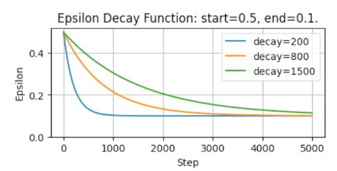
Epsilon Greediness - more exploration
Epsilon greediness lets the agent occasionally choose a random action over the highest value one. Decayed greediness can be followed to focus more on exploration early in training and more on exploitation later.
$\epsilon = end + (start - end) \cdot e^{-\frac{step}{decay}}$
This is implemented in the select_action() function -
it requires 5 arguments -
q_values: The Q-values for all actions in the current state. This determines the optimal action.step: the current step numberstart,endanddecay- thre parameters describing the epsilon decay.
# slect action based on decayed epsilon greedy method
def select_action(q_values, step, start, end, decay):
    # calculate the threshold value for this step
    epsilon = (end + (start-end)*math.exp(-step/decay))
    # draw a random number between 0 and 1
    sample = random.random()
    if sample < epsilon:
        # Return the random action index
        return random.choice(range(len(q_values)))
    #Return the action index with the highest Q value
    return torch.argmax(q_values).item()
Fixed Q value - more stable learning
The loss function is such that the target keeps changing with the network’s own predictions.
This is because -
- Q-network is used in both q-value and TD Target calculation
- this shifts both q-value and the target value.
This can lead to instability. To address this, we use a separate target network that is a copy of the main Q-network but with frozen weights. The target network is updated periodically (e.g., every few episodes) with the weights of the main Q-network. This way, the target values are more stable during training.
Target network
A target neural network predicts the target Q-values, and its weights are updated less frequently than the main network. This helps to stabilize training by providing a more consistent target for the loss function.
The online Q-network is updated every step, while the target network is updated every few episodes (or steps) by copying the weights from the online network.
Implementation
- Initialize the online and target networks with the same parameters.
# Initialize online and target networks with same initial parameters. online_network = QNetwork(8, 4) target_network = QNetwork(8,4) target_network.load_state_dict(online_network.state_dict()) -
Run gradient descent on the online network every step, to determine the q-values for all the states in the batch.
- Periodically not at every step, but once in a batch, update the target network weights and biases with that of the weighted average of that of the online network. This way, the target network is updated less frequently, providing more stable targets for the loss function.
A small valuetauis a hyperparameter that controls the update rate of the target network. A common choice istau = 0.001, which means that the target network is updated with 0.1% of the online network’s weights and 99% of its own weights at each update step.
def update_target_network(target_network, online_network, tau):
    target_net_state_dict = target_network.state_dict()
    online_net_state_dict = online_network.state_dict()
    for key in online_net_state_dict:
        target_net_state_dict[key] = (online_net_state_dict[key]*tau) + target_net_state_dict[key] * (1-tau)
    target_network.load_state_dict(target_net_state_dict)
    return None
- Training loop - the complete DQN algorithm with replay buffer, epsilon greedy action selection and target network update.
# 1. get the current state from environment
state, info = env.reset()

# 2. get the q-values for all the current states from the online network
q_values = online_network(state)

# 3. select action using epsilon greedy method
action = select_action(q_values, step, start, end, decay)

# 4. take action in the environment, get reward and next state
next_state, reward, done, info = env.step(action)

# 5. store the experience in replay buffer
replay_buffer.append((state, action, reward, next_state, done))

# 6. sample a batch of experiences from the replay buffer after replay buffer has enough samples
if len(replay_buffer) >= batch_size:
    batch = replay_buffer.sample(batch_size)

# 7. Identify the q_values of the current states and the actions taken in those states from the batch
q_values = online_network(states).gather(1, actions).squeeze(1)

# 8. compute the target Q-values using the target network. Don't compute gradients for the target network, as it is not being updated every step.
with torch.no_grad():
  # obtain the next state q_values across all columns in a given row
  next_state_q_values = target_network(next_states).amax(1)
  target_q_values = rewards + GAMMA * next_state_q_values * (1-dones)

# 9. compute the loss between the predicted Q-values from the online network and the target Q-values
loss = nn.MSELoss()(target_q_values, q_values)

# 10. perform a gradient descent step to update the online network's weights
optimizer.zero_grad()
loss.backward()
optimizer.step()

# 11. periodically update the target network's weights with that of the online network using a weighted average
update_target_network(target_network, online_network, tau)
Full implementation of the DQN algorithm with replay buffer, epsilon greedy action selection and target network update
"""
Greedy Epsilon and fix Q-value
"""

import gymnasium as gym
import matplotlib.pyplot as plt
import numpy as np
from datetime import datetime
import torch
import torch.nn as nn
import random
import math

from q_network import QNetwork
from replay_buffer import ReplayBuffer


GAMMA = 0.99
LR = 1e-4
NUM_EPISODES = 100
batch_size = 64
replay_buffer = ReplayBuffer(capacity=10000)
tau = 0.001

q_network = QNetwork(8, 4)
optimizer = torch.optim.Adam(q_network.parameters(), lr=LR)
criterion = nn.MSELoss()
online_network = QNetwork(8, 4)
target_network = QNetwork(8,4)
target_network.load_state_dict(online_network.state_dict())

def update_target_network(target_network, online_network, tau):
    target_net_state_dict = target_network.state_dict()
    online_net_state_dict = online_network.state_dict()
    for key in online_net_state_dict:
        target_net_state_dict[key] = (online_net_state_dict[key]*tau) + target_net_state_dict[key] * (1-tau)
    target_network.load_state_dict(target_net_state_dict)
    return None


# slect action based on decayed epsilon greedy method
def select_action(q_values, step, start, end, decay):
    # calculate the threshold value for this step
    epsilon = (end + (start-end)*math.exp(-step/decay))
    # draw a random number between 0 and 1
    sample = random.random()
    if sample < epsilon:
        # Return the random action index
        return random.choice(range(len(q_values)))
    #Return the action index with the highest Q value
    return torch.argmax(q_values).item()


def to_tensor(state):
    return torch.tensor(state, dtype=torch.float32)

def describe_episode(episode, reward, episode_reward, step, terminated, truncated, total_steps):
    if truncated:
        status = "Timeout"
    elif episode_reward >= 200:
        status = "Solved"
    elif episode_reward >= 100:
        status = "Landed"
    elif episode_reward >= 0:
        status = "Improving"
    elif episode_reward >= -100:
        status = "Stabilizing"
    else:
        status = "Crashed"

    print(
        f"| Episode {episode + 1:4d} | Duration: {step:4d} steps | Reward: {episode_reward:10.2f} | {status:<12} | Total Steps: {total_steps:6d} |"
    )


def plot_rewards(episode_rewards):
    episodes = list(range(1, len(episode_rewards) + 1))
    timestamp = datetime.now().strftime("%Y%m%d_%H%M%S")
    trend_filename = f"lunar_lander3_rewards_trend_{timestamp}.png"
    hist_filename = f"lunar_lander3_rewards_histogram_{timestamp}.png"
    x = np.asarray(episodes, dtype=np.float32)
    y = np.asarray(episode_rewards, dtype=np.float32)

    # Linear trend line: y = m*x + b
    m, b = np.polyfit(x, y, 1)
    trend = m * x + b

    # Line plot with trend line
    plt.figure(figsize=(10, 5))
    plt.plot(episodes, episode_rewards, color="tab:blue", linewidth=1.8, label="Episode Reward")
    plt.plot(episodes, trend, color="tab:red", linewidth=2.0, linestyle="--", label="Trend")
    plt.title("LunarLander Reward per Episode")
    plt.xlabel("Episode")
    plt.ylabel("Reward")
    plt.grid(alpha=0.3)
    plt.legend()
    plt.tight_layout()
    plt.savefig(trend_filename, dpi=150)

    # Histogram of achieved rewards
    plt.figure(figsize=(10, 5))
    plt.hist(episode_rewards, bins=15, color="tab:green", edgecolor="black", alpha=0.75)
    plt.title("Histogram of Episode Rewards")
    plt.xlabel("Reward")
    plt.ylabel("Frequency")
    plt.grid(alpha=0.25)
    plt.tight_layout()
    plt.savefig(hist_filename, dpi=150)
    print(f"Saved plots: {trend_filename}, {hist_filename}")

    plt.show()


env = gym.make("LunarLander-v3", render_mode="human")
all_episode_rewards = []
total_steps = 0
for episode in range(NUM_EPISODES):
    state, info = env.reset()
    done = False
    step = 0
    episode_reward = 0.0

    while not done:
        step += 1
        total_steps += 1
        # invokes the online_network and passes the inputs states, and it returns q_values for all the states - 1 row for each state.
        q_values = online_network(state)
        # select the action with epsilon greediness
        action = select_action(q_values, total_steps, start=0.9, end=0.05, decay=1000)
        # apply the chosen action to the environment for one timestep, till done.
        next_state, reward, terminated, truncated, _ = env.step(action)
        done = terminated or truncated

        # store the latest experience in the replay buffer.
        replay_buffer.push(state, action, reward, next_state, done)

        # sample a batch of 64 experiences from the replay buffer
        if len(replay_buffer) >= batch_size:
            states, actions, rewards, next_states, dones = replay_buffer.sample(batch_size)
            q_values = online_network(states).gather(1, actions).squeeze(1)
            # don't update the weights of the target network during backward propagation. gradients are not tracked.
            with torch.no_grad():
                # obtain the next state q_values across all columns in a given row
                next_state_q_values = target_network(next_states).amax(1)
                target_q_values = rewards + GAMMA * next_state_q_values * (1-dones)
            loss = nn.MSELoss()(target_q_values, q_values)
            optimizer.zero_grad()
            loss.backward()
            optimizer.step()
            update_target_network(target_network, online_network, tau=0.005)
        state = next_state
        episode_reward += reward

    all_episode_rewards.append(episode_reward)
    describe_episode(episode, reward, episode_reward, step, terminated, truncated, total_steps)

env.close()
plot_rewards(all_episode_rewards)
Double DQN - DDQN - to address overestimation bias in Q-learning
PLAIN DQN - Double Queue Network - With the target network separated out, it reduces feedback loops from rapidly moving target, but does not fully remove overestimation bias.
-
In DQN, there is a tendency to overestimate Q-values because the calculation of all target q_values involves taking maximum across all actions.This maximum is not taken from the real action value function, but from our current best estimate (from a neural network, that has not seen all the trainsitions yet), which is noisy.
-
In standard DQN, the target uses : $y = r + \gamma \max_{a’} Q_{\theta^-}(s’, a’)$
The issue is that Q-value function is being approximated by a neural network with parameters $\theta^-$, and the max operator is applied to these noisy estimates, which can lead to overestimation of the true Q-values.
In DQN target there are two parameter sets being used -
- $(Q_\theta)$: online network (being updated),
- $(Q_{\theta^-})$: target network (older/frozen copy for stability).
-
In tabular Bellman equations, one often write just (Q(s,a)) (no parameters), because each state-action has its own stored value.
-
This is known as
maximization biasoroverestimation biasin Q-learning. This leads to slower and less stable learning. -
For vanilla Q-learning, the update rule is - (Value Estimation)
\(\left[Q_1(s,a) \leftarrow (1-\alpha)Q_1(s,a) + \alpha\left[r + \gamma \max_{a'} Q_0(s',a')\right]\right]\)
- $(Q_1)$: online/current network (being updated).
- $(Q_0)$: target/frozen network (older copy).
- $(\alpha)$: learning rate.
- $(r + \gamma(\cdot))$: bootstrapped Bellman target.
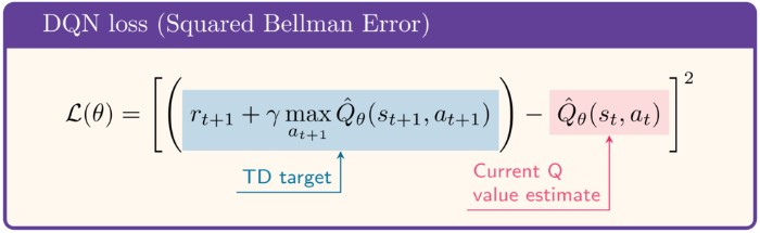
in NN training, this is implemented as minimizing the loss function :
\(\left[\big(Q_1(s,a)-[r+\gamma\max_{a'}Q_0(s',a')]\big)^2\right]\)
-
Action selection = choosing which next action looks best: $[a^*=\arg\max_{a’} Q_0(s’,a’)]$ - $max_a = argmax(Q_1(s’))$
- Value estimation = evaluating how good that chosen action is: $[Q_0(s’,a^*)]$
-
In vanilla DQN target: $[r + \gamma \max_{a’} Q_0(s’,a’)]$
- this is equivalent to:
- $(a^* = \arg\max_{a’} Q_0(s’,a’))$ (pick best action under $(Q_0)$) - action selection
- use $(Q_0(s’,a^))$ as the value - value estimation
Both these tasks are being done by the Target NN
So $(\max_{a’} Q_0(s’,a’) = Q_0(s’,a^))$.
Same thing, different notation. Vanilla formula hides the separate “select then evaluate” steps by writing them as one max expression.
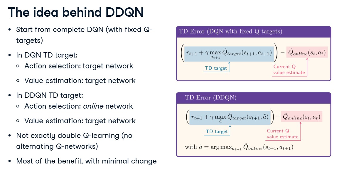
Double DQN - DDQN - This addresses overestimation more directly by decoupling selection and evaluation of the action in the target calculation.
$[a^* = \arg\max_{a’} Q_{\theta}(s’,a’) \quad\text{(select with online net)}]$
$[y = r + \gamma Q_{\theta^-}(s’, a^*) \quad\text{(evaluate with target net)}]$
DDQN - Double DQN Implementation
"""
Greedy Epsilon and fix Q-value
"""

import gymnasium as gym
import matplotlib.pyplot as plt
import numpy as np
from datetime import datetime
import os
import sys
import atexit
import csv
import torch
import torch.nn as nn
import random
import math

from q_network import QNetwork
from replay_buffer import ReplayBuffer


GAMMA = 0.99
LR = 1e-4
NUM_EPISODES = 100
batch_size = 64
replay_buffer = ReplayBuffer(capacity=10000)
tau = 0.001

q_network = QNetwork(8, 4)
optimizer = torch.optim.Adam(q_network.parameters(), lr=LR)
criterion = nn.MSELoss()
online_network = QNetwork(8, 4)
target_network = QNetwork(8,4)
target_network.load_state_dict(online_network.state_dict())


class Tee:
    def __init__(self, *streams):
        self.streams = streams

    def write(self, data):
        for stream in self.streams:
            stream.write(data)
        return len(data)

    def flush(self):
        for stream in self.streams:
            stream.flush()

    def isatty(self):
        return any(getattr(stream, "isatty", lambda: False)() for stream in self.streams)


def setup_console_file_logging():
    timestamp = datetime.now().strftime("%Y%m%d_%H%M%S")
    log_dir = "logs"
    os.makedirs(log_dir, exist_ok=True)
    log_path = os.path.join(log_dir, f"lunar_lander4_ddqn_{timestamp}.log")

    original_stdout = sys.stdout
    original_stderr = sys.stderr
    log_file = open(log_path, "a", encoding="utf-8")

    sys.stdout = Tee(original_stdout, log_file)
    sys.stderr = Tee(original_stderr, log_file)

    def _cleanup():
        sys.stdout = original_stdout
        sys.stderr = original_stderr
        log_file.close()

    atexit.register(_cleanup)
    print(f"Logging console output to: {log_path}")
    return log_path


def update_target_network(target_network, online_network, tau):
    target_net_state_dict = target_network.state_dict()
    online_net_state_dict = online_network.state_dict()
    for key in online_net_state_dict:
        target_net_state_dict[key] = (online_net_state_dict[key]*tau) + target_net_state_dict[key] * (1-tau)
    target_network.load_state_dict(target_net_state_dict)
    return None


# slect action based on decayed epsilon greedy method
def select_action(q_values, step, start, end, decay):
    # calculate the threshold value for this step
    epsilon = (end + (start-end)*math.exp(-step/decay))
    # draw a random number between 0 and 1
    sample = random.random()
    if sample < epsilon:
        # Return the random action index
        return random.choice(range(len(q_values)))
    #Return the action index with the highest Q value
    return torch.argmax(q_values).item()


def to_tensor(state):
    return torch.tensor(state, dtype=torch.float32)

def describe_episode(episode, reward, episode_reward, step, terminated, truncated, total_steps):
    if truncated:
        status = "Timeout"
    elif episode_reward >= 200:
        status = "Solved"
    elif episode_reward >= 100:
        status = "Landed"
    elif episode_reward >= 0:
        status = "Improving"
    elif episode_reward >= -100:
        status = "Stabilizing"
    else:
        status = "Crashed"

    print(
        f"| Episode {episode + 1:4d} | Duration: {step:4d} steps | Reward: {episode_reward:10.2f} | {status:<12} | Total Steps: {total_steps:6d} |"
    )
    return status


def plot_rewards(episode_rewards):
    episodes = list(range(1, len(episode_rewards) + 1))
    timestamp = datetime.now().strftime("%Y%m%d_%H%M%S")
    trend_filename = f"lunar_lander3_rewards_trend_{timestamp}.png"
    hist_filename = f"lunar_lander3_rewards_histogram_{timestamp}.png"
    x = np.asarray(episodes, dtype=np.float32)
    y = np.asarray(episode_rewards, dtype=np.float32)

    # Linear trend line: y = m*x + b
    m, b = np.polyfit(x, y, 1)
    trend = m * x + b

    # Line plot with trend line
    plt.figure(figsize=(10, 5))
    plt.plot(episodes, episode_rewards, color="tab:blue", linewidth=1.8, label="Episode Reward")
    plt.plot(episodes, trend, color="tab:red", linewidth=2.0, linestyle="--", label="Trend")
    plt.title("LunarLander Reward per Episode")
    plt.xlabel("Episode")
    plt.ylabel("Reward")
    plt.grid(alpha=0.3)
    plt.legend()
    plt.tight_layout()
    plt.savefig(trend_filename, dpi=150)

    # Histogram of achieved rewards
    plt.figure(figsize=(10, 5))
    plt.hist(episode_rewards, bins=15, color="tab:green", edgecolor="black", alpha=0.75)
    plt.title("Histogram of Episode Rewards")
    plt.xlabel("Reward")
    plt.ylabel("Frequency")
    plt.grid(alpha=0.25)
    plt.tight_layout()
    plt.savefig(hist_filename, dpi=150)
    print(f"Saved plots: {trend_filename}, {hist_filename}")

    plt.show()


setup_console_file_logging()
env = gym.make("LunarLander-v3", render_mode="human")
all_episode_rewards = []
total_steps = 0
timestamp = datetime.now().strftime("%Y%m%d_%H%M%S")
os.makedirs("logs", exist_ok=True)
csv_path = os.path.join("logs", f"lunar_lander4_ddqn_episode_summary_{timestamp}.csv")

with open(csv_path, "w", newline="", encoding="utf-8") as csv_file:
    csv_writer = csv.writer(csv_file)
    csv_writer.writerow(["episode", "duration", "reward", "state_name", "total_steps"])

for episode in range(NUM_EPISODES):
    state, info = env.reset()
    done = False
    step = 0
    episode_reward = 0.0

    while not done:
        step += 1
        total_steps += 1
        # invokes the online_network and passes the inputs states, and it returns q_values for all the states - 1 row for each state.
        q_values = online_network(state)
        # select the action with epsilon greediness
        action = select_action(q_values, total_steps, start=0.9, end=0.05, decay=1000)
        # apply the chosen action to the environment for one timestep, till done.
        next_state, reward, terminated, truncated, _ = env.step(action)
        done = terminated or truncated

        # store the latest experience in the replay buffer.
        replay_buffer.push(state, action, reward, next_state, done)

        # sample a batch of 64 experiences from the replay buffer
        if len(replay_buffer) >= batch_size:
            states, actions, rewards, next_states, dones = replay_buffer.sample(batch_size)
            q_values = online_network(states).gather(1, actions).squeeze(1)
            # don't update the weights of the target network during backward propagation. gradients are not tracked.
            with torch.no_grad():
                # obtain the next state q_values across all columns in a given row, for Q-target calculation
                next_actions = online_network(next_states).argmax(1).unsqueeze(1)
                # estimate next state q_values using the target network, and select the q_value corresponding to the next action selected by the online network.
                next_q_values = (target_network(next_states).gather(1, next_actions).squeeze(1))
                target_q_values = (rewards + GAMMA * next_q_values * (1-dones))
            loss = nn.MSELoss()(target_q_values, q_values)
            optimizer.zero_grad()
            loss.backward()
            optimizer.step()
            update_target_network(target_network, online_network, tau=0.005)
        state = next_state
        episode_reward += reward

    all_episode_rewards.append(episode_reward)
    state_name = describe_episode(episode, reward, episode_reward, step, terminated, truncated, total_steps)
    with open(csv_path, "a", newline="", encoding="utf-8") as csv_file:
        csv_writer = csv.writer(csv_file)
        csv_writer.writerow([episode + 1, step, f"{episode_reward:.2f}", state_name, total_steps])

env.close()
print(f"Saved episode CSV: {csv_path}")
plot_rewards(all_episode_rewards)
Summary
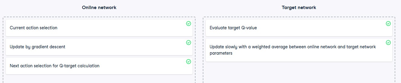
Online Network and Target Network:
- The online network is used for action selection and is updated by gradient descent.
- The target network is used for value evaluation and is updated by taking a weighted average between both networks.
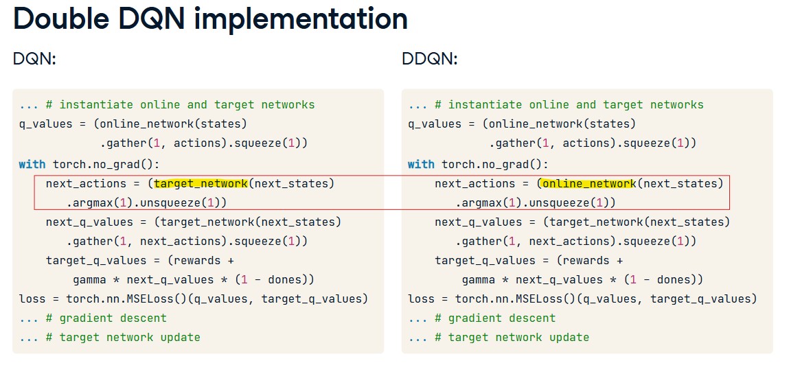
Training Double DQN:
- Use the online network to calculate actions for the Q-target calculation.
- Use the target network to estimate the Q-value corresponding to these actions.