Brief History of Deep Learning
Supervised learning
Since the advent of computers, scientists have been formulating ways to enable machines to take
input and produce desired output for tasks like classification and regression.
- Classification : Predicting a discrete label for an input. For example, predicting whether an email is spam or not. Or the sensor data is normal or not. This is made possible by training the model with labeled data - both normal and not normal.
- Regression : Predicts numerical values. For example, predicting the price of a house based on its features like size, location, etc.
These models are trained with a data set that is labeled already.
Unsupervised learning
In some cases where the labeled data is not available to train the model, the model finds structure in data without the knowledge of labels / classes ahead of time.
Early days
- Neural network were conceived in 1940s. The concept of backward propagation was introduced in 1960s. It was then neural networks were able to solve problems previously deemed unsolvable -
- image captioning
- language translation
- audio and video synthesis
- Today neural networks are primarily used for the following use cases -
- self-driving cars
- calculating risks,
- detecting frauds
- early cancer detection
What is a Artificial Neural Network?
- A network of artificial neurons.
- Here is one neuron -
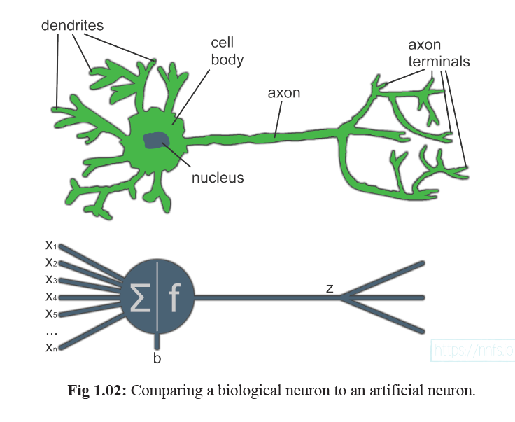
- A single neuron is relatively useless. But when combined with hundreds of thousands of neurons, the inter-connectivity produces relationships and results that frequently outperforms any other machine learning method.
Example neural networks
What is its purpose?
A neural network can be used to perform the following tasks -
- Classification - Predict a discrete label for an input. For example, predicting whether an email is spam or not. Or the sensor data is normal or not. This is made possible by training the model with labeled data - both normal and not normal.
- Regression - Predicts numerical values. For example, predicting the price of a house based on its features like size, location, etc.
- Clustering - Grouping similar data points together. For example, clustering customers based on their purchasing behavior.
The method of operation
This goal of the neural network is achieved by being able to transform the input data into a different nature of the output data using trial and error optimization techniques, with different parameters. The goal is to adjust those parameters to be able to get the desired transformation.
- Transform the input data into a different nature of output data. Typically the input data would belong to a vector space of a different nature than that of the expected output.
- Example : - Like for example, based on the sensor data (numerical), say it is needed to predict whether the sensor is about to fail in future (binary classification). The sensor data is a vector of numerical values, but the output is a binary value.
- This can be visually represented as follows -

- We typically do not know how the output would look like. So, we cannot define an algorithm to transform the input to the output, using a rule based method.
- So, in such cases neural network is used, where randomly we keep doing the following arbitrarily, repeatedly, till the difference between what is generated by the transformation and the expected output is on a decreasing trend.
- Change Size : Weights : Do linear transformation of the input vector, till it is either magnified or reduced to the desired output. For this weights are used.
- Change position : Bias : Change the origin, to be able place the magnified vector to a different vector space. For this biases are used.
- Change shape : Activation function : Change the shape of the vector to be able to fit into the desired output. For this activation function is used. This typically brings in non-linearity to the model.
| Purpose | Example | |
|---|---|---|
| Weights | Change size | Linear transformation of the input vector, till it is either magnified or reduced to the desired output. |
| Biases | Change position | Change the origin, to be able place the magnified vector to a different vector space. |
| Activation function | Change shape | Change the shape of the vector to be able to fit into the desired output. This typically brings in non-linearity to the model. |
Structure of a neural network
1. Neuron
- A neuron is a basic unit of a neural network.
- It takes inputs,
- applies weights and biases,
- and passes the result through an activation function to produce an output.
2. Interconnections of neurons
- Every neuron has one ore more inputs. And one or more outputs.
- One neuron connects with all the neurons of the next layer.
- The output of one neuron becomes the input to the next neuron.
3. Weights
- Each connection between neurons has a weight associated with it.
- It gets multiplied with the input to the neuron.
- Weights help to regulate the amount of the different inputs to be fed into a neuron. It is like different flavours of the different inputs are regulated to give a unique hint of each input, so that we get the desired output.
- The weights are trainable factors.
- It basically creates a linear combination of the inputs. That transforms the inputs to a different output vector, which might be more suitable for the real-world types of dynamic data.
- But it is still a linear transformation.

4. Bias
- Once the weighted sum of the inputs are calculated, a bias is added before passing through an activation function.
- The purpose of the bias is to offset the output positively or negatively, which can further help us map to the real-world types of dynamic data.
- This shifts the linear transformation done by the weights to a different unit vectors and hence new vector space.
- Bias is also trainable
5. Activation function
Activation function brings non linearity to the model. In its simplest form, it can be a step function, or it can be more complex function like ReLu etc.
The non linearity is brought about by being able to fire or not fire a neuron, based on the input information.
Examples of Activation Functions : Sigmoid, ReLU, Tanh, Softmax, etc.
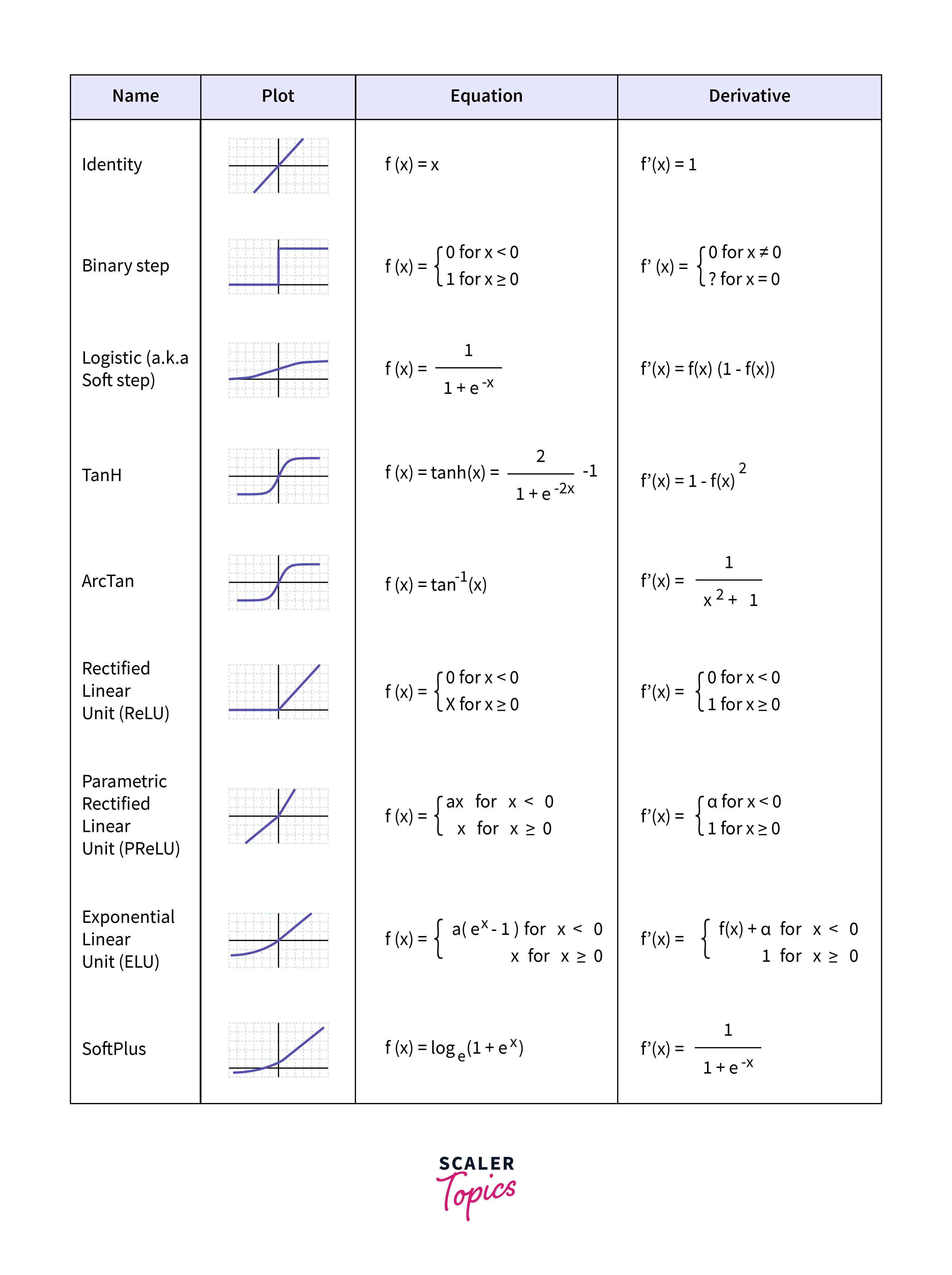
- step function - not able to predict how close the activation function is from activating or deactivating. surprises.
- relu - rectified linear unit. It is a piecewise linear function that will output the input directly if it is positive; otherwise, it will output zero. It is a very popular activation function in deep learning because it helps to mitigate the vanishing gradient problem.
Relu in work
Hidden layers activation functions
Activation functions will typically be same for all the hidden layers.
Output layer activation functions
6. Weights, biases and activation functions in action
Training of a neural network
What is trained?
To train these neural networks, we start with a random set of parameter matrices known as weight and biases, we calculate how “wrong” they are.
This amount of wrongness is called the loss. The attempt is to slowly adjust the weights and biases, so that over many iterations, the network gradually becomes, “less wrong”, i.e. the loss function is minimized.
- Weights - the strength of the connection between two neurons. The weights are adjusted during training to minimize the error in the model’s predictions. To begin with arbitrary random matrix for weights are taken.
- Bias - the bias is added to the weighted sum of inputs before passing it through the activation function. It allows the model to fit the data better by shifting the activation function to the left or right.
The goal of the training
Minimize the loss function
- The loss function measures how well the model’s predictions match the actual labels in the training data. The goal is to minimize this loss function by adjusting the weights and biases in the direction that reduces the error.
Generalization
The network should be able to see many examples of never-seen-before data, and accurately output values we hope to achieve.
How is it trained?
- A neural network outputs a concoction which has the right proportion of the input ingredients. The flavor of the concoction is determined by the right proportion of the input ingredients.
- To start with, an initial matrix of weights and an initial matrix of biases are taken. This is determined randomly.
- The output of the neuron is compared to the expected output (the label) using a loss function. The loss function measures how well the model’s predictions match the actual labels in the training data.
- The loss is then backpropagated through the network to update the weights and biases using an optimization algorithm (like gradient descent). The goal is to minimize the loss function by adjusting the weights and biases in the direction that reduces the error.
Why we get the right answer?
The physics of why a given prediction is made by the neural network is not known. It is a purely mathematical optimization problem based on expected and actual results.
Input of a neural network
- Normalization and Scaling - Inputs need to be in numeric form. The input data is is scaled to lie between 0 and 1 or -1 and 1.
Output of a neural network
Typically number of output states will be equal to the number of labels in the training set. If the number of labels is two, then the output can be one, indicating a binary number indicating presence of absence of the label.
Tracking down the maths and code of a neural network
A neural network has thousands or even upto millions of adjustable parameters (weights and biases). In this way, a neural network acts as enormous functions with vast number of parameters.
There exists some combination of these parameters that will yield the desired output. The end goal for a neural network is to adjust their parameters, so when applied to a yet unseen example as input, they produce a desired output.

Loss function
- argmax ()
- cross entropy
As we’ve already discussed, the example confidence level might look like [0.22, 0.6, 0.18] or [0.32, 0.36, 0.32]. In both cases, the argmax of these vectors will return the second class as the prediction, but the model’s confidence about these predictions is high only for one of them.
The Categorical Cross-Entropy Loss accounts for that and outputs a larger loss the lower the
confidence is: $L_i = -\log(\hat y_{i,k}) $ where k is the index of the true probability class. And $L_i$ denotes sample loss value for i-th sample in a set, k is the index of the target label (ground-true label). $y$ denotes the target value, and $\hat y$ is the predicted value.
Optimization algorithm
It is about adjusting weights and biases to minimize the loss function. The most common optimization algorithm is gradient descent. It works by calculating the gradient of the loss function with respect to the weights and biases, and then updating them in the opposite direction of the gradient.
Issues with Neural Networks
Overfitting
- Overfitting occurs when a model learns the training data too well, including its noise and outliers, leading to poor generalization to new data. This can happen when the model is too complex or when there is not enough training data.
- The algorithm only learns to fit the training data, but does not actually “understands” about the underlying input-output dependencies. The network basically just memorizes the training data.
Solving overfitting
- Use “out of sample” data to test the model. This is data that was not used in training the model.
- Use regularization techniques to penalize complex models. This can include L1 and L2 regularization, dropout, and early stopping.