Overview
GAN was there to convert a noise into image, by using two networks, generator and discriminator. The generator creates images from random noise, while the discriminator evaluates them. The two networks are trained together in a game-like process, where the generator tries to create images that fool the discriminator, and the discriminator tries to correctly identify real images from fake ones.
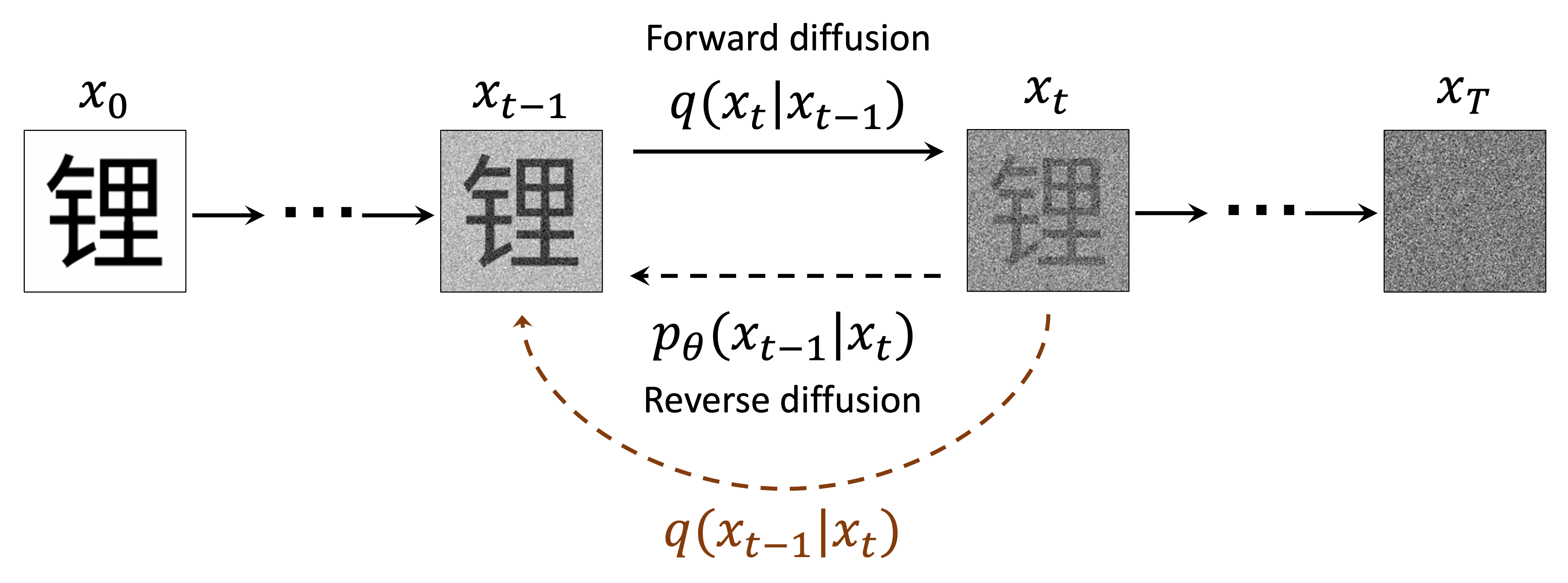
Diffusion models are a new class of generative models that have shown impressive results in generating high-quality images. They work by gradually adding noise to an image and then learning to reverse this process, effectively denoising the image step by step. This approach allows diffusion models to generate images with fine details and complex structures.
The idea is depicted in the video below
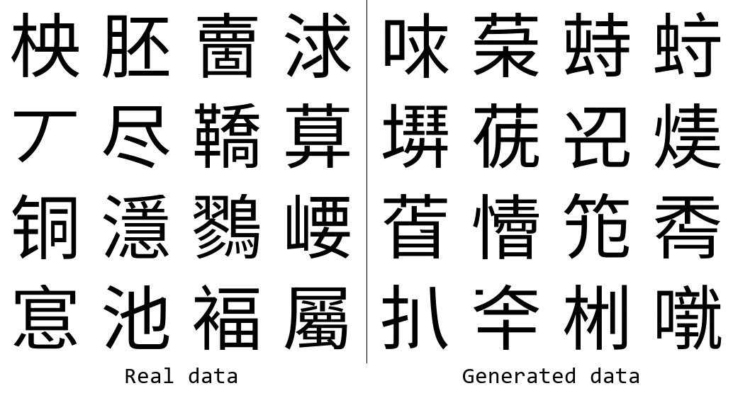
Task of generating chinese Glyphs
Pixel space
Words are projected into high dimension spaces using word embeddings. Similarly , images can also be projected into high dimensional spaces. Where, each point (vector) in the space represent an image. The vector space is known as pixel space.
An image is represented first in a pixel space. In RGB. It is a higher dimensional space. Each pixel is represented by three values (R, G, B). The image is a 3D tensor of size (height, width, 3).
if each picture is of the pixel size 128x128, then each image can be represented as a fixed length vector of size 128x128 = 16384. If each of these vectors are denoted as a point, that space with all these points is known as pixel space.
![]()
We can call the domain of all possible images for our dataset “pixel space”.
Reduction of dimensionality
The pixel space is very high dimensional. It is difficult to work with such high dimensional data. So, we need to reduce the dimensionality of the pixel space. As per the manifold hypothesis natural datasets lie on lower dimensional manifolds embedded in a higher dimensional space. Dimensional reduction techniques like UMAP - uniform manifold approximation and projection can be used to project our data set from 16384 dimensions to 2 dimensions. The 2D projection retains lots of structure, consistent with the that our data lie on a lower dimensional manifold embedded in the pixel space.
Images belonging to one category form a cluster in the pixel space. In the 2D UMAP of the pixel space for the chinese characters, below, there are two clusters. Left cluster is for chinese characters that are horizontally stacked, and the right cluster is for chinese characters that are vertically stacked.
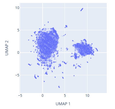
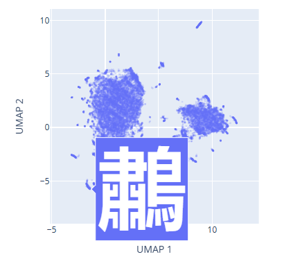
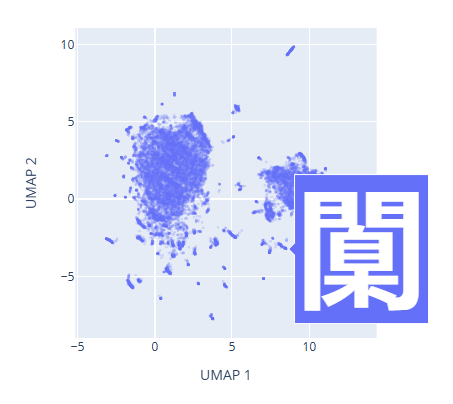
Image as a probability distribution
If images are converted into numbers, and they belong to a probability distribution space, then we can use the probability distribution to generate new images. The idea is to learn the underlying probability distribution of the data, and then sample from it to generate new images.
So, given the training images, those are converted into a pixel space. The goal is to predict the probability distribution of the data in the pixel space. This is determined via supervised learning. Once the probability distribution is learned, we can sample from it to generate new images.
1. A simple intuition of a 1D Gaussian distribution
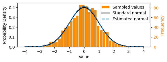
- Consider the one-dimensional normal (Gaussian) distribution above, commonly written $X \sim \mathcal{N}(μ,σ^2)$, where $X$ is a random variable, $μ$ is the mean, and $σ2$ is the variance. The normal distribution is a continuous probability distribution that is symmetric about its mean.
- Let it be parameterized with mean $μ=0$ and variance $σ^2=1$. The black curve above shows the probability density function of the normal distribution.
- We can sample from it: drawing values such that over a large number of samples, the set of values reflects the underlying distribution. These days, we can simply write something like x = random.gauss(0, 1) in Python to sample from the standard normal distribution, although the computational sampling process itself is non-trivial!
- We could think of a set of numbers sampled from the above normal distribution as a simple dataset, like that shown as the orange histogram above.
- In this particular case, we can calculate the parameters of the underlying distribution using maximum likelihood estimation, i.e. by working out the mean and variance.
- The normal distribution estimated from the samples is shown by the dotted line above.
Effectively we have learnt an underlying probability distribution form the data.
2. Image Data representation
- The image dataset used for the glyffuser model is ~21,000 pictures of Chinese glyphs. The images are all the same size, 128 × 128 = 16384 pixels, and greyscale (single-channel color). Thus an obvious choice for the representation is a vector $\vec x$ of length 16384, where each element corresponds to the brightness of one pixel.
x of length 16384, where each element corresponds to the color of one pixel $\vec x = (x_1,x_2,x_3,…,x_{16384})$. The domain of all possible images for our dataset can be called as pixel space
An example glyph with pixel values labelled (downsampled to 32 × 32 pixels for readability).
![]()
3. Visualizing the image dataset
-
Imagine that the individual data samples $\vec x$, are actually sampled from an underlying probability distribution $q(x)$, in a pixel space, much as the samples from the Gaussian distribution above were sampled from a normal distribution. $x \sim q(x)$
-
In the case of Gaussian distribution, we could parameterize the distribution $q(x)$ with a mean and variance, and then sample from it, using MLE - maximum likelihood estimation to estimate the parameters of the distribution. In the case of image data set, since the imagined distribution is very high dimensional, we cannot use MLE. Instead, machine learning is used to learn the parameters of the distribution.
-
As an approximation, we can visualize the probability distribution of the real data set as a 2D UMAP projection of the pixel space. The UMAP projection is a non-linear dimensionality reduction technique that preserves the local structure of the data. The UMAP projection of the pixel space for the glyffuser dataset is shown below.
-
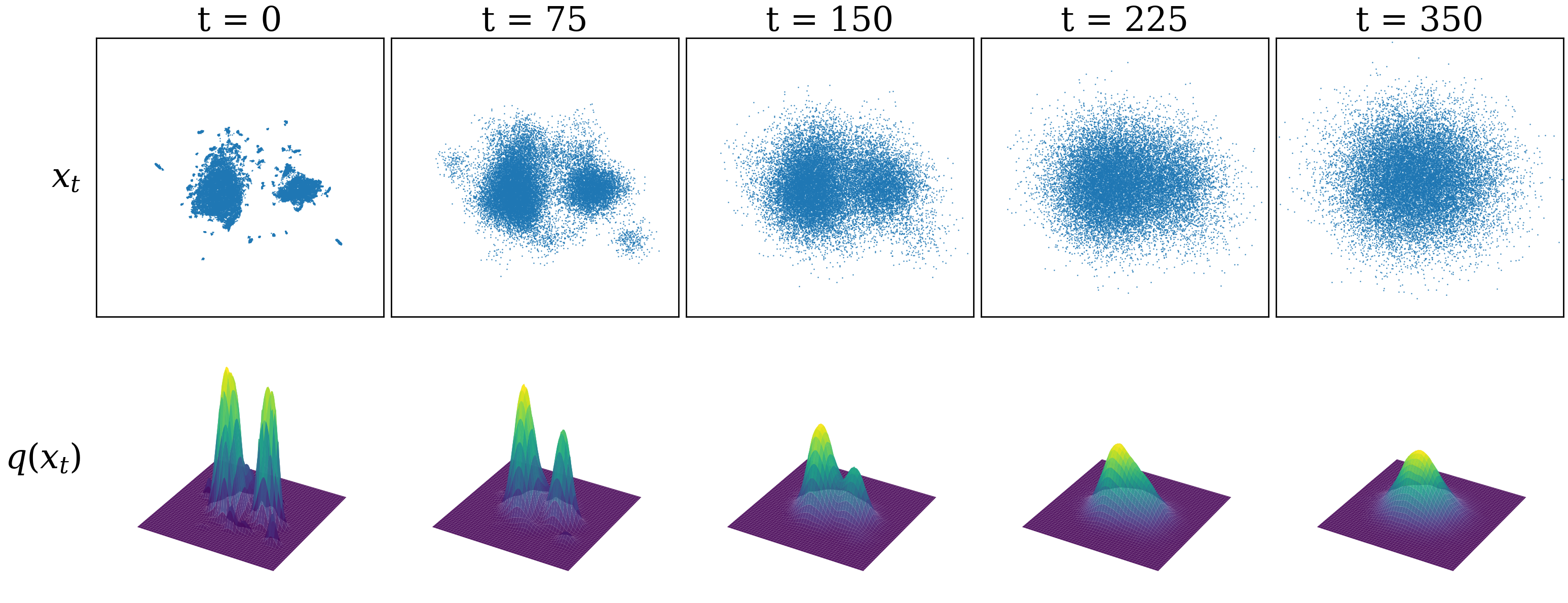
Let’s now use this low-dimensional UMAP dataset as a visual shorthand for our high-dimensional dataset. Remember, we assume that these individual points have been sampled from a continuous underlying probability distribution $x \sim q(x)$. To get a sense of what this distribution might look like, we can apply a KDE (kernel density estimation) over the UMAP dataset. (Note: this is just an approximation for visualization purposes)
At the green peaks of the probability distributions, there is highest probability of finding the chinese glyphs. The plain area are the noise. The whole process of generating image is basically traversing all the way to the peak and sampling the glyphs from the pixel space, corresponding to the peak.
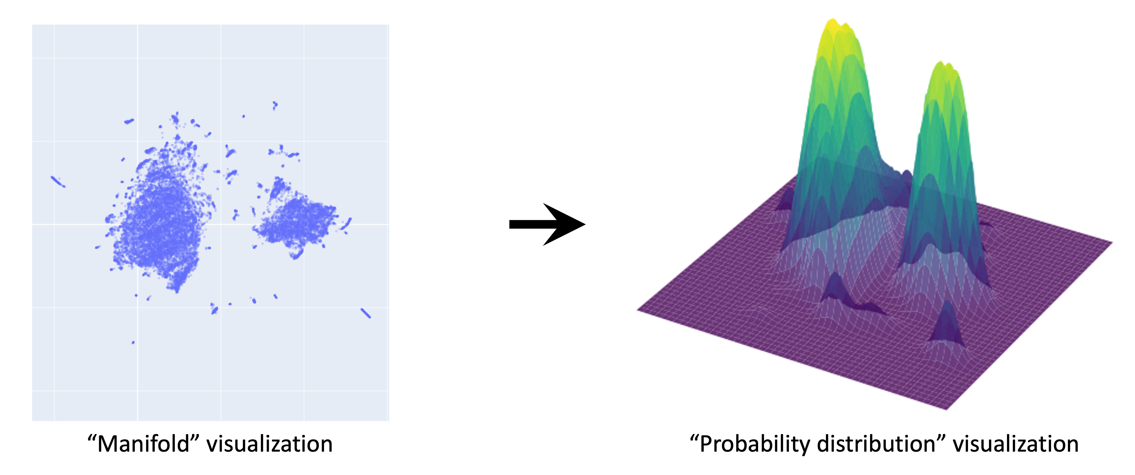
This gives a sense of what $x \sim q(x)$ should look like: clusters of glyphs correspond to high-probability regions of the distribution. The true q(x) lies in 16384 dimensions—this is the distribution we want to learn with our diffusion model.
We showed that for a simple distribution such as the 1-D Gaussian, we could calculate the parameters (mean and variance) from our data. However, for complex distributions such as images, we need to call on ML methods. Moreover, what we will find is that for diffusion models in practice, rather than parameterizing the distribution directly, they learn it implicitly through the process of learning how to transform noise into data over many steps.
This is illustrated below to determine the picture of a bear
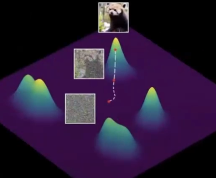
There might be such clusters of all the images in the corpus.
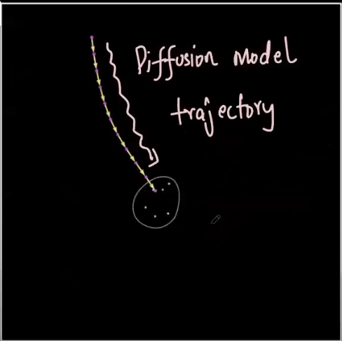
- Such probability distributions intuitively enables the algorithm to find the patterns in the pixel space of the training data where “good” images live. The diffusion model actually searches through the empty spaces in the pixel space (noise), to determine a trajectory to the actual good image. This trajectory is defined by the machine learning.
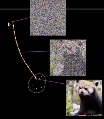
Here the probability distribution is important because it quantifies the likelihood of finding more number of good images in the pixel space. This aids the diffusion model to quantify the existence of the images, where the model needs to navigate
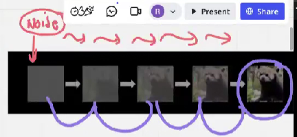
Gradual denoising
Diffusion models have recently come into the spotlight as a particularly effective method for learning these probability distributions. They generate convincing images by starting from pure noise and gradually refining it
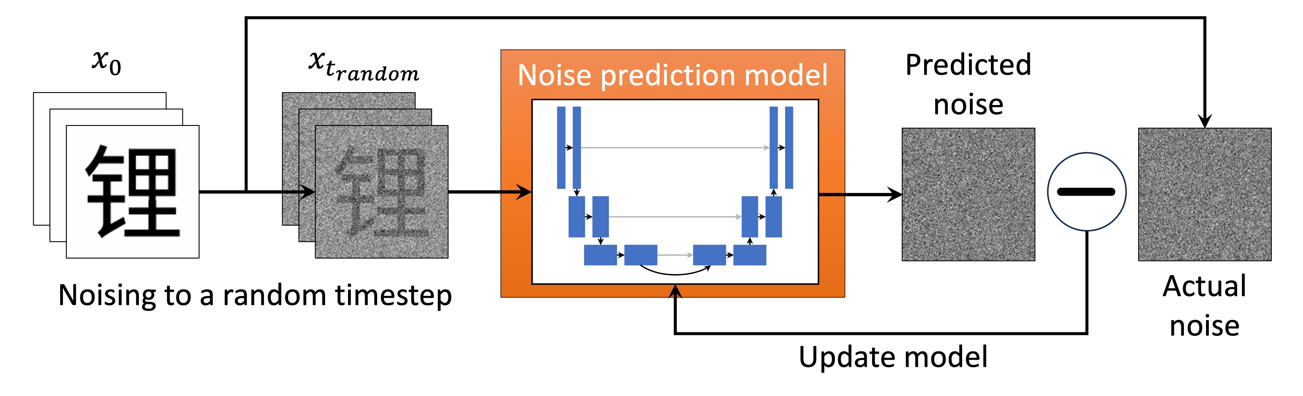
Steps of the diffusion model
Step 1 : Take an image
Step 2 : Generate random noise
Step 3 : Select random time step
Step 4 : Use noise scheduler to add noise
The below is the noise scheduling scheme
\(\text{noisy\_image} = \sqrt{\alpha_t} \cdot x_0 + \sqrt{1 - \alpha_t} \cdot \text{noise}\)
$\alpha_t$ goes on decreasing with time.
$x_0$ is the original image.
Step 5 : Noise prediction
The noisy image is sampled from step 4, and is passed through the ML model to train it to predict noise in that image.
Step 6 : Backward propagation and update model parameters
Step 7 : Run this for many iterations.
Eventually the model learns precisely how the image gets noisier at each time step. And then successfully reverse the process.
References
Research papers
- Denoising Diffusion Probabilistic Models - Ho et al. (2020)
- Diffusion Models Beat GANs on Image Synthesis - Dhariwal and Nichol (2021)
- Transfusion: Text-to-Image Generation using Cross-Modal Diffusion - Chen et al. (2022)
- Transfusion: Predict the next token and diffuse images with one multi modal model
- Photorealistic Text-to-Image Diffusion Models with Deep Language Understanding - Saharia et al. (2022)
Online blogs
- chinese dataset visualization
- online image generator
- Google Imagen
- diffusion model book - chinese dataset visualization
- diffusion model code for chines letters generation
- further reading
Courses
- stanford deep generative model