Diffusion model for Devanagari script generation

Devanagari Script Generation Diffusion Model Analysis

Executive Summary

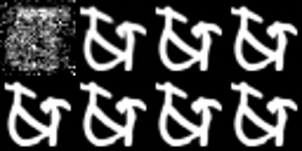
This report presents a comprehensive analysis of a diffusion model designed for generating Devanagari script characters. The model successfully generates high-quality Devanagari characters after just 2 epochs of training on a dataset of 92,000 images. This document outlines the model’s architecture, examines the current configuration, and proposes optimization strategies to enhance performance while maintaining generation quality.

1. Introduction to Diffusion Models

Diffusion models represent a powerful class of generative models that learn to reverse a gradual noising process. The process begins with adding noise to images until they become pure noise, then training the model to reverse this process step by step. For Devanagari script generation, this approach is particularly suitable due to the complex structure and intricate details of the characters.

1.1 Diffusion Model Theory

Diffusion models are based on two key processes:

1. Forward Process (Diffusion): A Markov chain that gradually adds Gaussian noise to the data over T timesteps
2. Reverse Process (Denoising): A learned process that gradually removes noise to recover the data distribution

1.2 Diffusion Pipeline Stages

The complete diffusion model pipeline consists of:

1. Data Preparation: Preprocessing the Devanagari script images
2. Forward Diffusion: Adding predetermined noise to training images
3. Model Training: Learning to predict and remove noise
4. Sampling: Generating new Devanagari characters through iterative denoising
5. Post-processing: Enhancing the generated images if needed

2. Detailed Model Architecture Analysis

2.1 Core Architecture

The implemented diffusion model uses a U-Net architecture with the following key components:

2.1.1 U-Net Architecture Breakdown

The U-Net architecture consists of:

1. Input Layer:
   • Accepts 32×32 pixel images
   • Processes the noise level embedding (timestep)
   • Initial convolution to map to the feature space
2. Encoder Path:
   • Sequential downsampling blocks that progressively reduce spatial dimensions
   • Feature maps become deeper as they become spatially smaller
   • Downsampling operations: convolutions with stride 2
   • 6 downsampling stages with channel dimensions [128, 128, 256, 256, 512, 512]
3. Bottleneck:
   • Middle blocks with highest feature depth (512 channels)
   • Contains self-attention layers for global information processing
   • Captures highest-level abstract features of the Devanagari script
4. Decoder Path:
   • Sequential upsampling blocks that restore spatial dimensions
   • Feature maps become shallower as they expand spatially
   • Upsampling operations: transposed convolutions or upsample + convolution
   • 6 upsampling stages mirroring the encoder path
   • Skip connections from encoder to decoder for preserving detailed information
5. Skip Connections:
   • Connect corresponding layers in encoder and decoder
   • Allow detailed spatial information to bypass the bottleneck
   • Essential for preserving fine details in the generated Devanagari characters
6. Time Embedding:
   • Processes the diffusion timestep using sinusoidal positional embeddings
   • Transformed through MLPs to condition each block’s operation
   • Allows the model to adapt its behavior based on the denoising stage
7. Output Layer:
   • Final convolution to map features to the output space
   • Produces noise prediction to guide the denoising process

2.2 Block Configuration

The model implements a sophisticated block structure:

2.2.1 Downsampling Blocks (Encoder)

The implementation uses six down blocks with increasing feature dimensions:

block_out_channels=(128, 128, 256, 256, 512, 512)
down_block_types=(
    "DownBlock2D",
    "DownBlock2D",
    "DownBlock2D",
    "DownBlock2D",
    "AttnDownBlock2D",
    "DownBlock2D",
)

Each DownBlock2D typically contains:

• ResNet-style blocks with convolutions, normalization, and activations
• Spatial downsampling via strided convolutions
• Timestep embedding injection through adaptive normalization or addition

The AttnDownBlock2D additionally contains:

• Self-attention mechanisms operating on feature maps
• Enables the model to capture relationships between different parts of the characters
• Particularly important for maintaining structural coherence in complex scripts

2.2.2 Upsampling Blocks (Decoder)

The upsampling path contains six blocks:

up_block_types=(
    "UpBlock2D",
    "AttnUpBlock2D",
    "UpBlock2D",
    "UpBlock2D",
    "UpBlock2D",
    "UpBlock2D",
)

Each UpBlock2D typically contains:

• ResNet-style blocks with convolutions, normalization, and activations
• Spatial upsampling via transposed convolutions or upsampling + convolution
• Skip connection integration from corresponding encoder blocks
• Timestep embedding injection

The AttnUpBlock2D additionally contains:

• Self-attention mechanisms similar to the encoder path
• Helps maintain global coherence during the upsampling process

2.3 Attention Mechanism In-Depth

The attention blocks implement a mechanism similar to the transformer’s self-attention:

1. Query, Key, Value Projections:
   • Features are projected into query (Q), key (K), and value (V) spaces
   • Projections are performed using learned convolutional layers
2. Attention Computation:
   • Scaled dot-product attention: Attention(Q,K,V) = softmax(QK^T/√d)V
   • Allows the model to focus on relevant features across the spatial domain
3. Multi-Head Implementation:
   • Multiple attention heads operating in parallel
   • Each head captures different relationship patterns
   • Outputs are concatenated and projected back to the original feature space

This attention mechanism is crucial for capturing the intricate relationships between different strokes and components of Devanagari characters.

2.4 Time Conditioning

Time conditioning is fundamental to diffusion models:

1. Timestep Embedding:
   • Converts scalar timestep t to a high-dimensional embedding using sinusoidal functions
   • Embedding dimension is typically 4 times the base channel dimension
2. MLP Projection:
   • Processes the embedding through a small MLP network
   • Transforms the embedding into format suitable for modulating the U-Net blocks
3. Feature Modulation:
   • Injected into each block through adaptive normalization or additive bias
   • Controls how each layer processes features based on the denoising stage

This time conditioning allows the model to adapt its behavior based on the noise level, which is critical for the progressive denoising process.

3. Training Configuration Analysis

3.1 Current Configuration

class TrainingConfig:
    image_size = 32  # assumes images are square
    train_batch_size = 32
    eval_batch_size = 32
    num_epochs = 2  # Reduced from 20 to 2
    gradient_accumulation_steps = 1
    learning_rate = 1e-4
    lr_warmup_steps = 500
    save_image_epochs = 1
    save_model_epochs = 30
    mixed_precision = "fp16"
    output_dir = output_folder
    overwrite_output_dir = True
    seed = 0
    dataset_name = "data128"

3.2 Optimizer and Scheduler

• Optimizer: Adam - efficient stochastic optimization with adaptive learning rates
• Scheduler: Cosine schedule with warmup - gradually increases learning rate during initial training, then decreases it following a cosine curve

3.3 Performance Insights

The model achieving good results after just 2 epochs (reduced from 20) suggests:

• The dataset of 92,000 images provides sufficient examples for learning
• The model architecture is well-suited for the task
• The complexity of Devanagari script generation might be lower than initially anticipated
• The chosen hyperparameters create an efficient learning environment

4. Industry Best Practices for Diffusion Model Optimization

4.1 Efficient Training with Limited Data

4.1.1 Data Augmentation Strategies

Effective data augmentation is crucial when working with limited training data:

1. Geometric Transformations:
   • Rotation: Small rotations (±5-10°) preserve character integrity while adding variety
   • Slight Scaling: Scale variations (0.9-1.1x) increase robustness
   • Translation: Small shifts preserve local patterns
   • Flipping: Should be used carefully for script data as it may affect readability
2. Appearance Transformations:
   • Brightness/Contrast: Subtle adjustments simulate different writing conditions
   • Elastic Deformations: Gentle warping imitates different writing styles
   • Noise Injection: Adding small amounts of structured noise before the diffusion process
3. Script-Specific Augmentations:
   • Stroke Width Variation: Simulate different pen widths
   • Component Recombination: For compound characters, mix components from different samples
   • Style Transfer: Apply minor style changes across characters

Implementation Example:

def augment_devanagari(image):
    # Geometric transformations
    angle = random.uniform(-5, 5)
    scale = random.uniform(0.95, 1.05)
    image = tf.image.rot90(image, k=angle/90)
    
    # Appearance transformations
    image = tf.image.random_brightness(image, max_delta=0.1)
    image = tf.image.random_contrast(image, lower=0.9, upper=1.1)
    
    # Script-specific transformations
    # Implement custom transforms based on Devanagari structure
    
    return image

4.1.2 Latent Diffusion Models

Industry has moved toward latent diffusion models to improve efficiency:

1. Perceptual Compression:
   • Use a pre-trained VAE/autoencoder to compress images to a latent space
   • Perform diffusion in the compressed latent space rather than pixel space
   • Significantly reduces computational requirements while preserving quality
2. Implementation Process:
   • Train or use a pre-trained encoder-decoder model
   • Encode training images to latent representations
   • Train diffusion model on these latent codes
   • During generation, decode the latent samples to produce images
3. Benefits for Limited Data:
   • Reduced dimensionality means fewer parameters to learn
   • More efficient learning from limited examples
   • Better generalization properties

4.2 Noise Schedule Optimization

The noise schedule critically impacts model performance:

1. Linear vs. Cosine Schedules:
   • Linear schedules: Simple but often sub-optimal
   • Cosine schedules: Better preservation of low-frequency information
   • Sigmoid schedules: Can help balance early and late stage denoising
2. Learned Variance Schedules:
   • Allow the model to learn optimal noise schedules during training
   • Particularly effective for specialized domains like script generation
3. Noise Schedule for Script Generation:
   • Early denoising steps: Focus on overall character structure
   • Middle steps: Develop major strokes and components
   • Late steps: Refine details and connections between strokes

Industry Best Practice: Implement a “warm-start” noise schedule that preserves more structure in early diffusion steps:

def cosine_beta_schedule(timesteps, s=0.008):
    """
    Cosine schedule as proposed in Improved DDPM paper
    """
    steps = timesteps + 1
    x = torch.linspace(0, timesteps, steps)
    alphas_cumprod = torch.cos(((x / timesteps) + s) / (1 + s) * torch.pi * 0.5) ** 2
    alphas_cumprod = alphas_cumprod / alphas_cumprod[0]
    betas = 1 - (alphas_cumprod[1:] / alphas_cumprod[:-1])
    return torch.clamp(betas, 0.0001, 0.9999)

4.3 Advanced Conditioning Techniques

Conditioning the diffusion model improves performance with limited data:

1. Classifier Guidance:
   • Use a pre-trained classifier to guide the generation process
   • Steer the diffusion sampling toward regions with high classifier confidence
   • Implementation: Modify the score function with classifier gradients
2. Classifier-Free Guidance:
   • Train the model to work both with and without conditioning
   • During inference, interpolate between conditional and unconditional predictions
   • More efficient than classifier guidance and doesn’t require a separate classifier
3. Conditioning Types for Script Generation:
   • Character Identity: Condition on the character class/ID
   • Style Parameters: Condition on style indicators (thickness, slant)
   • Context Characters: Condition on neighboring characters for sequence generation

Code Example for Classifier-Free Guidance:

def sample_with_cfg(model, x, t, class_labels, cfg_scale=3.0):
    # Predict noise with conditioning
    noise_cond = model(x, t, class_labels)
    
    # Predict noise without conditioning (null conditioning)
    noise_uncond = model(x, t, None)
    
    # Combine predictions using CFG
    noise_pred = noise_uncond + cfg_scale * (noise_cond - noise_uncond)
    
    return noise_pred

4.4 Training Efficiency Techniques

Industry has developed several techniques to improve training efficiency:

1. Progressive Distillation:
   • Train a teacher model with many diffusion steps
   • Distill knowledge into a student model with fewer steps
   • Allows for high-quality generation with fewer inference steps
2. Offset Noise Optimization:
   • Introduce small offsets to the noise prediction target
   • Helps the model focus on the most informative aspects of the signal
   • Particularly useful for detailed features in scripts
3. Prediction Targets:
   • Predict the noise directly (ε-prediction)
   • Predict the denoised image (x₀-prediction)
   • Predict velocity (v-prediction)
   • Industry finding: v-prediction often works best for detailed structures
4. Efficient Attention Mechanisms:
   • Linear attention mechanisms reduce computational complexity
   • Sparse attention focuses on the most relevant portions of the feature maps
   • Memory-efficient attention implementations for larger batch sizes

Example Implementation of v-prediction:

def v_prediction_loss(model, x_0, t, noise):
    # Add noise to image according to timestep
    x_t = q_sample(x_0, t, noise)
    
    # Calculate velocity target
    alpha_t = extract(alphas_cumprod, t, x_0.shape)
    sigma_t = extract(sqrt_one_minus_alphas_cumprod, t, x_0.shape)
    v_target = alpha_t * noise - sigma_t * x_0
    
    # Predict v
    v_pred = model(x_t, t)
    
    # Calculate loss
    return F.mse_loss(v_pred, v_target)

4.5 Loss Function Specialization

Specialized loss functions improve training with limited data:

1. Perceptual Losses:
   • Incorporate losses based on pre-trained feature extractors
   • Emphasize perceptually important features of the script
   • Example: Use features from a CNN trained on script recognition
2. Structural Losses:
   • Incorporate losses that emphasize structural integrity
   • Example: Use SSIM (Structural Similarity Index) as a component of the loss
3. Adversarial Losses:
   • Incorporate a discriminator network for adversarial training
   • Can improve visual quality and adherence to the script style
4. Focal Loss Variants:
   • Adapt the standard MSE loss to focus more on difficult-to-predict regions
   • Particularly useful for intricate details in Devanagari characters

Industry Best Practice: Combine multiple loss components with appropriate weighting:

def combined_loss(model_output, target, perceptual_extractor, alpha=1.0, beta=0.1):
    # Standard diffusion loss
    mse_loss = F.mse_loss(model_output, target)
    
    # Perceptual loss
    perceptual_features_pred = perceptual_extractor(model_output)
    perceptual_features_target = perceptual_extractor(target)
    perceptual_loss = F.mse_loss(perceptual_features_pred, perceptual_features_target)
    
    # Combine losses
    total_loss = mse_loss + alpha * perceptual_loss
    
    return total_loss

5. Optimization Strategies for the Model

5.1 Architecture Optimizations

5.1.1 Block Configuration Refinement

Current Configuration:

block_out_channels=(128, 128, 256, 256, 512, 512)

Potential Optimizations:

• Graduated Channel Scaling: Implement a more gradual increase in channel dimensions

  block_out_channels=(64, 128, 192, 256, 384, 512)
  

• Balanced Attention Blocks: Distribute attention blocks more evenly

  down_block_types=(
      "DownBlock2D",
      "DownBlock2D",
      "AttnDownBlock2D",
      "DownBlock2D",
      "AttnDownBlock2D",
      "DownBlock2D",
  )
  up_block_types=(
      "UpBlock2D",
      "AttnUpBlock2D",
      "UpBlock2D",
      "AttnUpBlock2D",
      "UpBlock2D",
      "UpBlock2D",
  )
  

5.1.2 Resolution Considerations

The current 32×32 resolution may be limiting detail capture. Consider:

• Increasing to 64×64 for better detail preservation
• Implementing a multi-scale approach with additional blocks:

  block_out_channels=(64, 128, 192, 256, 384, 512, 512)
  

5.2 Training Optimizations

5.2.1 Learning Rate Tuning

• Learning Rate Range Test: Implement a test to find optimal learning rate range
• Cyclic Learning Rates: Consider implementing instead of cosine annealing

  learning_rate = 5e-5  # Lower base learning rate
  # With cyclic scheduler implementation
  

5.2.2 Batch Size Adjustments

• Batch Size Increase: If hardware allows, increase batch size for more stable gradients

  train_batch_size = 64  # Up from 32
  eval_batch_size = 64
  

• Gradient Accumulation: Increase steps for virtual batch size increase

  gradient_accumulation_steps = 4  # Up from 1
  

5.2.3 Advanced Regularization

• Dropout: Add dropout layers to prevent overfitting
• Data Augmentation: Implement rotation, slight scaling, and minor distortions

5.3 Noise Schedule Optimization

• Custom Noise Schedule: Implement a noise schedule tailored to Devanagari features
• Progressive Distillation: Train subsequent models with fewer diffusion steps

6. Evaluation Metrics and Monitoring

6.1 Quality Assessment

• FID (Fréchet Inception Distance): Implement to measure generated image quality
• Character Recognition Accuracy: Test with OCR systems to ensure legibility
• Human Evaluation: Conduct studies with Devanagari readers

6.2 Performance Monitoring

• Training Dynamics: Track loss curves during training
• Inference Speed: Measure generation time per character
• Model Size vs. Quality: Evaluate quality against model size tradeoffs

7. Conclusion and Recommendations

The current diffusion model for Devanagari script generation demonstrates remarkable efficiency by producing high-quality results after just 2 epochs. This suggests that:

1. The architecture is well-aligned with the complexity of the task
2. The dataset provides comprehensive coverage of Devanagari characters
3. The optimization strategy effectively navigates the solution space

Key Recommendations:

1. Short-term Improvements:
   • Experiment with balanced attention blocks
   • Implement targeted data augmentation
   • Test lower learning rates (3e-5 to 8e-5)
2. Medium-term Enhancements:
   • Increase image resolution to 64×64
   • Implement custom noise scheduling
   • Add conditional generation capabilities
3. Long-term Research Directions:
   • Explore knowledge distillation to create smaller models
   • Implement classifier-free guidance to improve generation quality
   • Develop specialized loss functions for Devanagari script characteristics

By implementing these recommendations systematically, the model can be further optimized for efficiency, quality, and versatility in Devanagari script generation.

Output:

Architecture of diffusion model

flowchart TD subgraph "Training Process" direction TB A[Input Image x₀] --> B[Forward Diffusion Process] B -->|"Add Noise (t steps)"| C[Noisy Image xₜ] C --> D[U-Net Model] T[Timestep t] --> D D --> E[Predicted Noise ε_θ] N[Actual Noise ε] --> F E --> F[Loss Calculation] F -->|Backpropagation| D end subgraph "U-Net Architecture" direction TB D1[Input: xₜ + t] --> D2[Initial Convolution] D2 --> E1[Encoder Path] subgraph "Encoder Path" direction TB E1 --> E2[DownBlock2D\n128 channels] E2 --> E3[DownBlock2D\n128 channels] E3 --> E4[DownBlock2D\n256 channels] E4 --> E5[DownBlock2D\n256 channels] E5 --> E6[AttnDownBlock2D\n512 channels] E6 --> E7[DownBlock2D\n512 channels] end E7 --> M1[Middle Block\nAttention + ResNet] M1 --> U1[Decoder Path] subgraph "Decoder Path" direction TB U1 --> U2[UpBlock2D\n512 channels] U2 --> U3[AttnUpBlock2D\n512 channels] U3 --> U4[UpBlock2D\n256 channels] U4 --> U5[UpBlock2D\n256 channels] U5 --> U6[UpBlock2D\n128 channels] U6 --> U7[UpBlock2D\n128 channels] end U7 --> O1[Output Convolution] O1 --> O2[Noise Prediction] %% Skip connections E2 -.->|Skip Connection| U6 E3 -.->|Skip Connection| U5 E4 -.->|Skip Connection| U4 E5 -.->|Skip Connection| U3 E6 -.->|Skip Connection| U2 end subgraph "Generation Process" direction TB G1[Random Noise xT] --> G2[Reverse Diffusion Process] G2 -->|"Denoise Step by Step"| G3[Generated Image x₀] G4[U-Net Model θ] --> G2 end %% Connect the processes D -.-> G4

Code base:

Code base for the implementation of the diffusion model to generate Devangari Scripts

Training configuration

class TrainingConfig:
    image_size = 32  # assumes images are square
    train_batch_size = 32
    eval_batch_size = 32
    num_epochs = epochs
    gradient_accumulation_steps = 1
    learning_rate = 1e-4
    lr_warmup_steps = 500
    save_image_epochs = 1
    save_model_epochs = 30
    mixed_precision = "fp16"  # `no` for float32, `fp16` for automatic mixed precision
    output_dir = output_folder  # the model name
    overwrite_output_dir = True  # overwrite the old model when re-running the notebook
    seed = 0
    dataset_name="data128"

config = TrainingConfig()

Training the model

def train_loop(config, model, noise_scheduler, optimizer, train_dataloader, lr_scheduler):
    accelerator = Accelerator(
        mixed_precision=config.mixed_precision,
        gradient_accumulation_steps=config.gradient_accumulation_steps,
        log_with="tensorboard",
        project_dir=os.path.join(config.output_dir, "logs")
    )

    if accelerator.is_main_process:
        if config.output_dir is not None:
            os.makedirs(config.output_dir, exist_ok=True)
        accelerator.init_trackers("train_example")

    model, optimizer, train_dataloader, lr_scheduler = accelerator.prepare(
        model, optimizer, train_dataloader, lr_scheduler
    )

    global_step = 0

    for epoch in range(config.num_epochs):
        progress_bar = tqdm(total=len(train_dataloader), disable=not accelerator.is_local_main_process)
        progress_bar.set_description(f"Epoch {epoch}")

        for step, batch in enumerate(train_dataloader):
            clean_images = batch
            noise = torch.randn(clean_images.shape).to(clean_images.device)
            bs = clean_images.shape[0]
            timesteps = torch.randint(0, noise_scheduler.num_train_timesteps, (bs,), device=clean_images.device).long()
            noisy_images = noise_scheduler.add_noise(clean_images, noise, timesteps)

            with accelerator.accumulate(model):
                noise_pred = model(noisy_images, timesteps, return_dict=False)[0]
                loss = F.mse_loss(noise_pred, noise)
                accelerator.backward(loss)
                accelerator.clip_grad_norm_(model.parameters(), 1.0)
                optimizer.step()
                lr_scheduler.step()
                optimizer.zero_grad()

            progress_bar.update(1)
            logs = {"loss": loss.detach().item(), "lr": lr_scheduler.get_last_lr()[0], "step": global_step}
            progress_bar.set_postfix(**logs)
            accelerator.log(logs, step=global_step)
            global_step += 1

        if accelerator.is_main_process:
            if (epoch + 1) % config.save_image_epochs == 0 or epoch == config.num_epochs - 1:
                pipeline = DDPMPipeline(unet=accelerator.unwrap_model(model), scheduler=inference_scheduler)
                evaluate(config, epoch, pipeline)

            if (epoch + 1) % config.save_model_epochs == 0 or epoch == config.num_epochs - 1:
                pipeline = DDPMPipeline(unet=accelerator.unwrap_model(model), scheduler=inference_scheduler)
                save_dir = os.path.join(config.output_dir, f"epoch{epoch}")
                pipeline.save_pretrained(save_dir)

Define the U-Net architecture

# Define model
model = UNet2DModel(
    sample_size=config.image_size,  # the target image resolution
    in_channels=1,  # the number of input channels
    out_channels=1,  # the number of output channels
    layers_per_block=1,  # how many ResNet layers to use per UNet block
    block_out_channels=(128, 128, 256, 256, 512, 512),  # the number of output channels for each UNet block
    down_block_types=(
        "DownBlock2D",
        "DownBlock2D",
        "DownBlock2D",
        "DownBlock2D",
        "AttnDownBlock2D",
        "DownBlock2D",
    ),
    up_block_types=(
        "UpBlock2D",
        "AttnUpBlock2D",
        "UpBlock2D",
        "UpBlock2D",
        "UpBlock2D",
        "UpBlock2D",
    ),
)

Define optimizer and schduler

noise_scheduler = DDPMScheduler(num_train_timesteps=1000)
# noise_scheduler = DDIMScheduler(num_train_timesteps=1000)
inference_scheduler = DPMSolverMultistepScheduler()
optimizer = AdamW(model.parameters(), lr=config.learning_rate)
lr_scheduler = get_cosine_schedule_with_warmup(
    optimizer=optimizer,
    num_warmup_steps=config.lr_warmup_steps,
    num_training_steps=(len(train_dataloader) * config.num_epochs),
)

Run the training on the model and generate the images

from accelerate import notebook_launcher

args = (config, model, noise_scheduler, optimizer, train_dataloader, lr_scheduler)
notebook_launcher(train_loop, args, num_processes=1)

model_path = output_folder + "/epoch" + output_folder_prefix  # Path to the specific epoch model directory# Path to the model directory
pipeline = DDPMPipeline.from_pretrained(model_path).to("cuda")
pipeline.scheduler = DPMSolverMultistepScheduler()

# Sample from the model and save the images in a grid
images = pipeline(
    batch_size=16,
    generator=torch.Generator(device='cuda').manual_seed(config.seed), # Generator can be on GPU here
    num_inference_steps=50
).images

# Make a grid out of the inverted images
image_grid = make_grid(images, rows=4, cols=4)

# Save the images
test_dir = os.path.join(config.output_dir, "samples")
os.makedirs(test_dir, exist_ok=True)
image_grid.save(f"{test_dir}/samples.png")

Visualize the images

from diffusers import DPMSolverMultistepScheduler, DDPMPipeline
from PIL import Image, ImageDraw, ImageFont
import torch

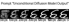
def make_labeled_grid(images, prompt, steps, font_path=None, font_size=20, margin=10):
    assert len(images) == len(steps), "The number of images must match the number of steps"

    w, h = images[0].size
    font = ImageFont.truetype(font_path, font_size) if font_path else ImageFont.load_default()

    # Calculate the height of the grid including the margin for text
    total_height = h + margin + font_size
    total_width = w * len(images)
    grid_height = total_height + margin + font_size  # Add extra margin for the prompt
    grid = Image.new('RGB', size=(total_width, grid_height), color=(255, 255, 255))
    # Draw the text prompt at the top
    draw = ImageDraw.Draw(grid)
    prompt_text = f"Prompt: \"{prompt}\""
    prompt_width, prompt_height = draw.textbbox((0, 0), prompt_text, font=font)[2:4]
    prompt_x = (total_width - prompt_width) / 2
    prompt_y = margin / 2
    draw.text((prompt_x, prompt_y), prompt_text, fill="black", font=font)

    for i, (image, step) in enumerate(zip(images, steps)):
        # Calculate position to paste the image
        x = i * w
        y = margin + font_size

        # Paste the image
        grid.paste(image, box=(x, y))

        # Draw the step text
        step_text = f"Steps: {step}"
        text_width, text_height = draw.textbbox((0, 0), step_text, font=font)[2:4]
        text_x = x + (w - text_width) / 2
        text_y = y + h + margin / 2 - 8
        draw.text((text_x, text_y), step_text, fill="black", font=font)
    return grid

# Initialize the model pipeline using your local model
model_path = output_folder + "/epoch" + output_folder_prefix  # Path to your trained model
pipeline = DDPMPipeline.from_pretrained(model_path).to("cuda")
pipeline.scheduler = DPMSolverMultistepScheduler()

# Define the number of steps to visualize
num_inference_steps_list = [1, 2, 3, 5, 10, 20, 50]

images = []

# Generate images for each value in num_inference_steps_list
for num_steps in num_inference_steps_list:
    generated_images = pipeline(
        batch_size=1,
        generator=torch.Generator(device='cuda').manual_seed(0),
        num_inference_steps=num_steps
    ).images
    images.append(generated_images[0])  # Append the generated image

# Create the labeled grid with a descriptive prompt since this is an unconditional model
prompt = "Unconditional Diffusion Model Output"
image_grid = make_labeled_grid(images, prompt, num_inference_steps_list)

# Show the grid
from IPython.display import display
display(image_grid)

# Save the image grid
image_grid.save("diffusion_steps_visualization3.png")

Create an animated visualization of the diffusion process

from diffusers import DPMSolverMultistepScheduler, DDPMPipeline
from PIL import Image, ImageDraw, ImageFont
import torch
import numpy as np
import os
import imageio.v2 as imageio
from tqdm import tqdm

# Initialize the model pipeline using your local model
model_path = output_folder + "/epoch" + output_folder_prefix  # Path to your trained model
pipeline = DDPMPipeline.from_pretrained(model_path).to("cuda")
pipeline.scheduler = DPMSolverMultistepScheduler()

# Create output directory for frames
os.makedirs("animation_frames", exist_ok=True)

# Set parameters
num_inference_steps = 50
seed = 42

# Use the model's forward process to generate images at each step
print("Generating denoising frames...")

# Start with pure noise (t=1000)
generator = torch.Generator(device="cuda").manual_seed(seed)

# Store all frames
frames = []

# The correct way to visualize the denoising process is to use the pipeline with
# increasing numbers of denoising steps
for step in tqdm(range(0, num_inference_steps + 1, 2)):  # Skip some steps for faster generation
    if step == 0:
        # For the initial noise, just use the pipeline with 1 step
        # This will effectively show the noise
        current_step = 1
    else:
        current_step = step

    # Generate the image with the current number of denoising steps
    image = pipeline(
        batch_size=1,
        generator=torch.Generator(device="cuda").manual_seed(seed),
        num_inference_steps=current_step
    ).images[0]

    # Save the frame
    image.save(os.path.join("animation_frames", f"frame_{step:03d}.png"))
    frames.append(image)

# Create GIF from frames
print("Creating GIF animation...")
# Ensure all frames have the same size (shouldn't be necessary but just in case)
frames_resized = [frame.resize((256, 256)) for frame in frames]

# Save as GIF
output_gif = "diffusion_process3.gif"
frames_resized[0].save(
    output_gif,
    save_all=True,
    append_images=frames_resized[1:],
    optimize=False,
    duration=150,  # milliseconds per frame - slower to see the changes
    loop=0  # 0 means loop indefinitely
)

print(f"Animation saved to {output_gif}")

# Create a grid showing selected frames
def create_process_grid(frames, num_to_show=8):
    # Select frames evenly throughout the process
    if len(frames) <= num_to_show:
        selected_frames = frames
    else:
        indices = np.linspace(0, len(frames)-1, num_to_show, dtype=int)
        selected_frames = [frames[i] for i in indices]

    # Resize frames
    width, height = 256, 256
    selected_frames = [frame.resize((width, height)) for frame in selected_frames]

    # Create grid image
    cols = min(4, num_to_show)
    rows = (num_to_show + cols - 1) // cols

    grid = Image.new('RGB', (width * cols, height * rows))

    for i, frame in enumerate(selected_frames):
        row = i // cols
        col = i % cols
        grid.paste(frame, (col * width, row * height))

    return grid

# Create and save the grid
grid = create_process_grid(frames)
grid.save("diffusion_process_grid3.png")
print("Process grid saved to diffusion_process_grid3.png")

Transfusion

Transfusion paper

CLIP : Image embeddings

CLIP image embeddings Vizuara - multi modal embeddings unsloth-ai

References

1. Ho, J., Jain, A., & Abbeel, P. (2020). Denoising diffusion probabilistic models. Advances in Neural Information Processing Systems.
2. Nichol, A., & Dhariwal, P. (2021). Improved denoising diffusion probabilistic models. International Conference on Machine Learning.
3. Rombach, R., Blattmann, A., Lorenz, D., Esser, P., & Ommer, B. (2022). High-resolution image synthesis with latent diffusion models. Proceedings of the IEEE/CVF Conference on Computer Vision and Pattern Recognition.
4. Saharia, C., Chan, W., Saxena, S., Li, L., et al. (2022). Photorealistic text-to-image diffusion models with deep language understanding. Advances in Neural Information Processing Systems.
5. Song, Y., Sohl-Dickstein, J., Kingma, D. P., Kumar, A., Ermon, S., & Poole, B. (2021). Score-based generative modeling through stochastic differential equations. International Conference on Learning Representations.
6. Dhariwal, P., & Nichol, A. (2021). Diffusion models beat GANs on image synthesis. Advances in Neural Information Processing Systems.
7. Karras, T., Aittala, M., Laine, S., Härkönen, E., Hellsten, J., Lehtinen, J., & Aila, T. (2022). Elucidating the design space of diffusion-based generative models. Advances in Neural Information Processing Systems.